Kronecker Structure in Composed Convolutions
20 Apr 2026 - Raúl Santiago Molina
This post is a technical note I’ve been sitting on since around 2019. At the time I was exploring what happens when you look at stacked convolutional layers as a single linear operation, and I noticed that the resulting virtual matrix has a very specific algebraic structure: it is a Kronecker product. Not because you choose to decompose it that way, but because it just is one, by construction.
I never published this as a formal paper or explored it further, as I got busy with work. Then, when a paper using Kronecker factorization appeared as an ICLR 2021 Outstanding Paper, I got excited: the same mathematical object I had been studying from the analysis side was being used on the design side for parameter-efficient layers. That coincidence motivated my earlier blog post about why Kronecker products are so effective. I ended that post saying the Kronecker product would be “a crucial tool in the path to understanding Neural Networks.” This post is the follow-through on that claim.
Now seemed like a good time to finally clean this up and write it out. Full disclosure: the code refactoring, visualizations, and much of the prose in this post were written with the help of Claude Code. The ideas and the original implementation are mine from 2019-2020; the presentation has been significantly improved by our collaboration. The analysis also includes a connection to gradient saliency maps that Claude spotted during our work together (thanks Claude!).
Kronecker Factorization of Images
Before connecting any of this to neural networks, let’s build some visual intuition for what a Kronecker decomposition actually does. The idea is simple: given a matrix \(A\) (say, a grayscale image), find two smaller matrices \(B\) and \(C\) such that their Kronecker product \(B \otimes C\) approximates \(A\):
\[A \approx B \otimes C\]The Kronecker product \(B \otimes C\) creates a block matrix where each element of \(B\) scales a copy of \(C\). So \(B\) controls the coarse structure (which blocks go where and how bright they are), while \(C\) controls the fine detail within each block.
The rearrangement trick
How do we find \(B\) and \(C\)? The key insight (Van Loan & Pitsianis, 1993) is that if we split the image into a grid of blocks, flatten each block into a vector, and stack those vectors as rows of a new matrix, the SVD of that rearranged matrix directly gives us the Kronecker factors.
The animation below shows this process step by step. Each patch is extracted from the original image (left, replaced by black) and its flattened pixels fill a row of the rearranged matrix (right):
The left singular vectors of this rearranged matrix give us \(B\), and the right singular vectors give us \(C\). The Kronecker decomposition is equivalent to SVD on the rearranged matrix.
Factor shapes: trading off structure and detail
The dimensions of \(B\) and \(C\) are constrained: their product must equal the original image dimensions (\(320 \times 480\)). But within that constraint, you can choose how to allocate the “budget” between them. Use the sliders below to explore. Notice how \(B\) and \(C\) always multiply to give the full image size:
B: 16 x 30 ⊗ C: 20 x 16 = 320 x 480
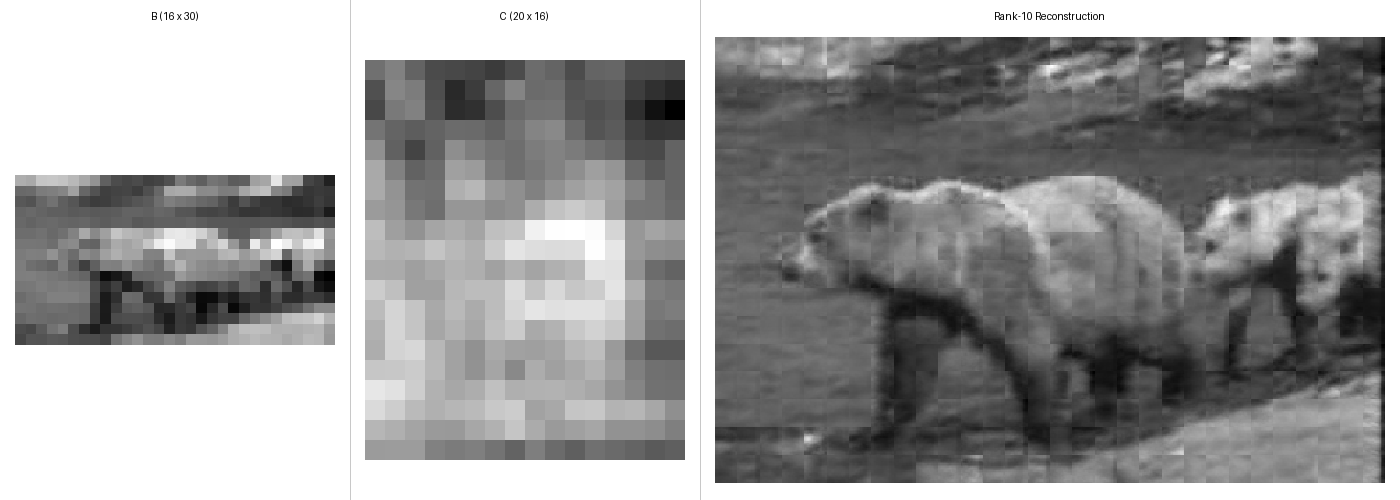
Notice the trade-off: a larger \(B\) captures more spatial detail (the bear’s shape is sharper), but \(C\) becomes tiny and can only hold coarse intensity patterns. A smaller \(B\) makes the reconstruction blockier, but \(C\) has more room for local texture. The product of their dimensions is always the original image size, a fixed budget that you allocate between coarse structure and fine detail.
Rank: how many terms you need
A single \(B \otimes C\) term (rank 1) gives a rough approximation. Adding more terms \(\sum_{i=1}^{r} B_i \otimes C_i\) captures increasingly fine detail, just like adding more singular values in SVD. Use the slider to see the effect:
![]()
At rank 1 the image is a single blocky pattern. By rank 10 the bear is clearly recognizable. By rank 50 it’s nearly indistinguishable from the original. Each additional rank adds one independent “mode” of variation, one more way the pixels can co-vary across the image.
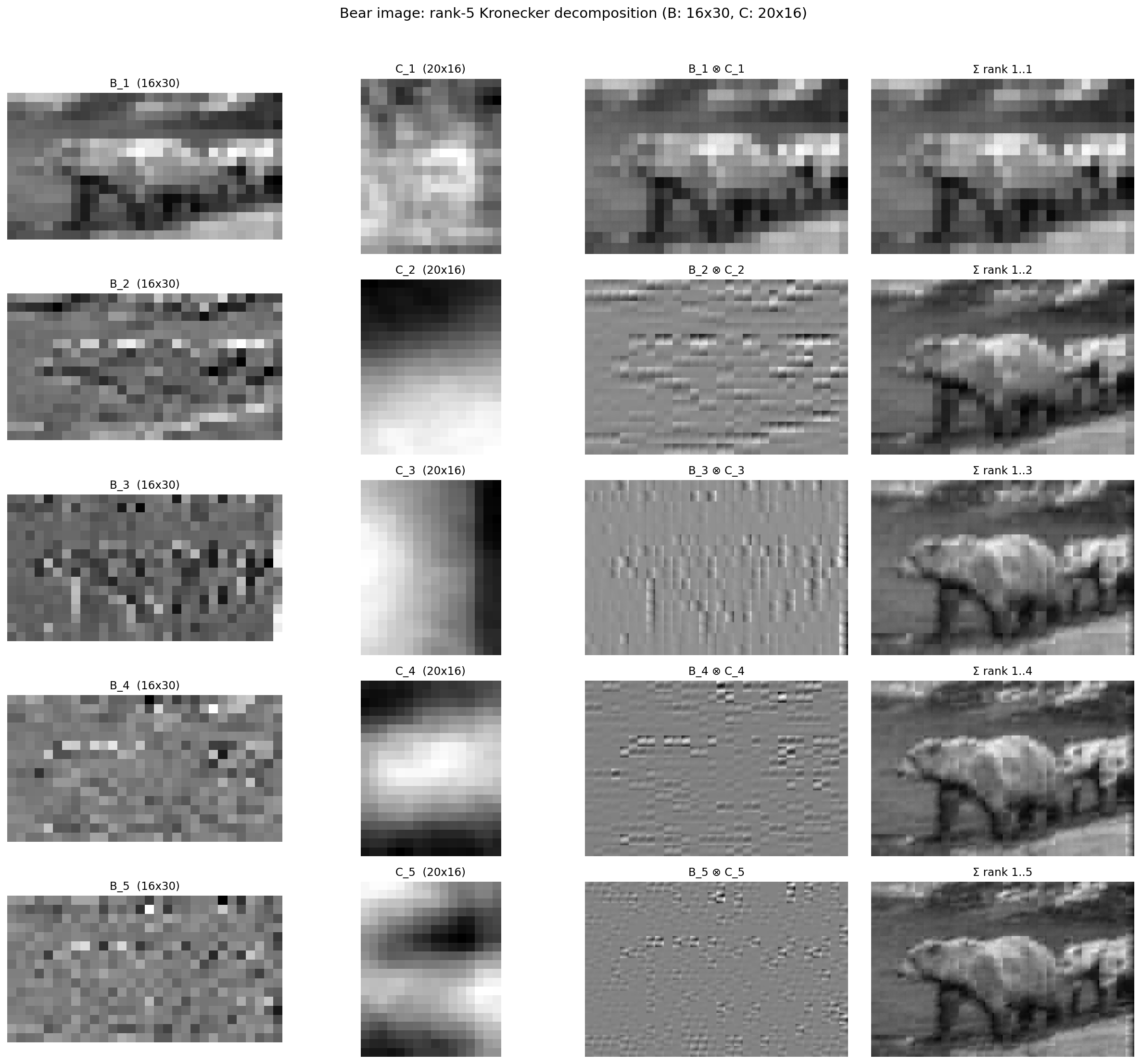
Looking at the individual factors at rank 5 reveals what each mode captures. The first mode accounts for global intensity (the overall brightness pattern of the bear against the background). The second and third modes pick up horizontal and vertical edges. The fourth captures finer line structure, and the fifth adds texture. Each row below shows \(B_i\), \(C_i\), their Kronecker product \(B_i \otimes C_i\), and the cumulative reconstruction up to that rank:
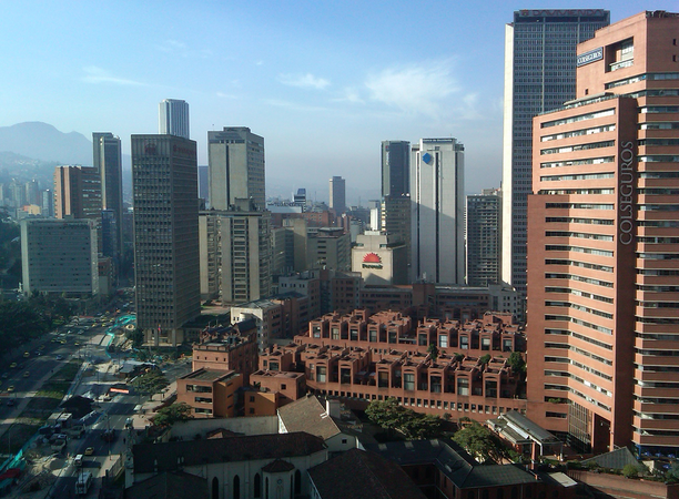
Color images: where does color live?
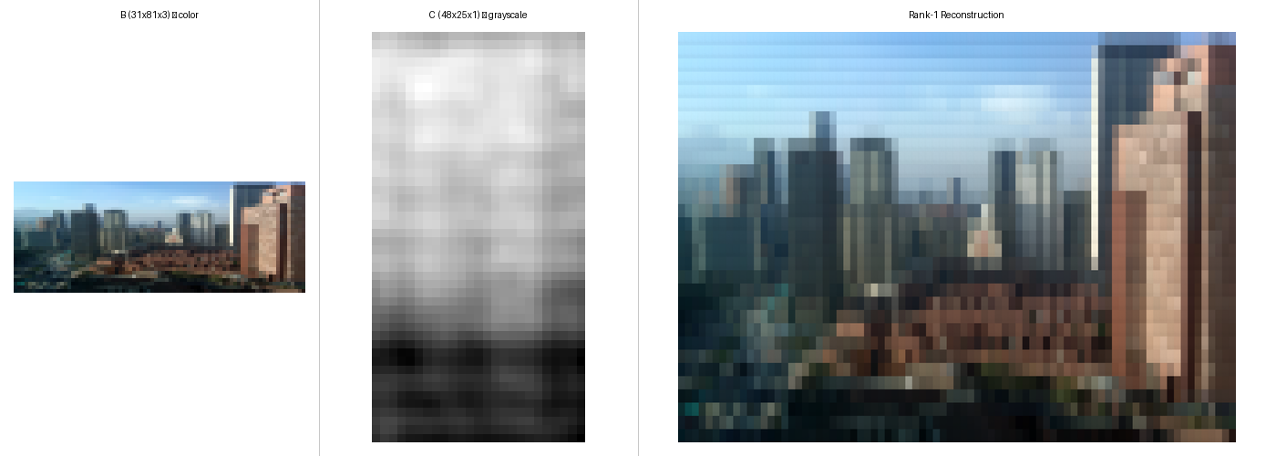
Everything so far has been grayscale. For a color image (here’s one of my hometown, Bogota) the 3 color channels can be assigned to either \(B\) (the coarse factor) or \(C\) (the detail factor):
To isolate this effect, we use a single Kronecker term (rank 1):
Color in \(B\), where each block has its own color and detail is grayscale:
Color in \(C\), where blocks are grayscale and color is applied uniformly within each block:
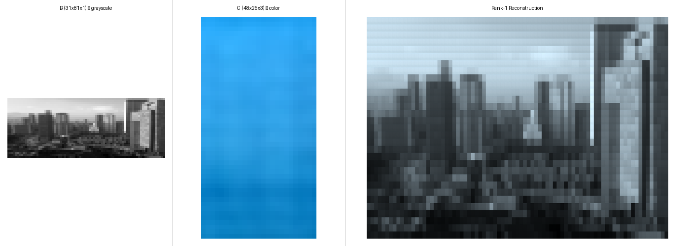
With color in \(B\), \(B_1\) is a small color thumbnail and \(C_1\) adds grayscale spatial detail, so the reconstruction has spatially varying color. With color in \(C\), \(B_1\) captures grayscale structure and \(C_1\) holds a single global color tint applied uniformly to every block. At higher ranks, additional terms can recover more color variation in both cases, but the rank-1 comparison makes clear where the color “budget” is allocated.
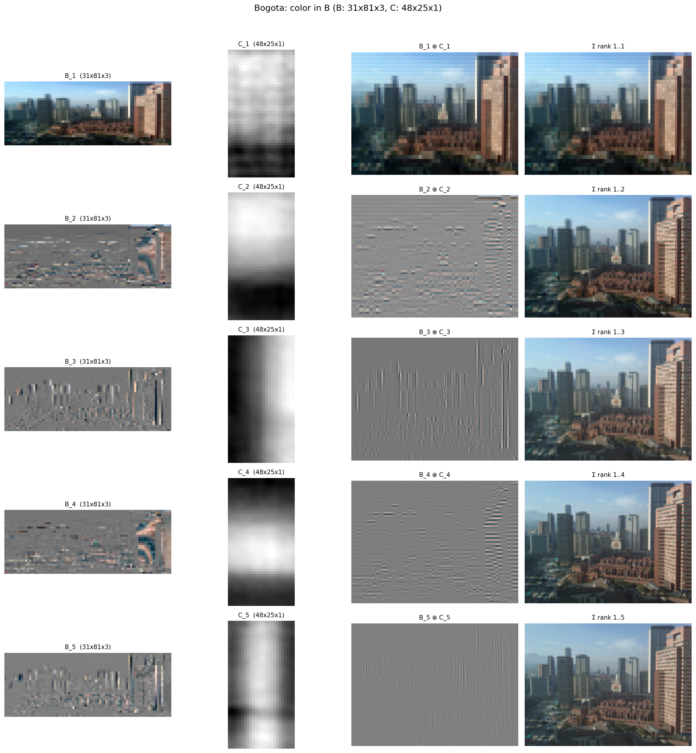
The rank-5 decomposition makes this even clearer. With color in \(B\), the story is similar to the grayscale bear: the first mode captures global intensity and color, while subsequent modes add edges, lines, and texture. The color information is “spent” in the first term, and the remaining modes refine spatial detail:
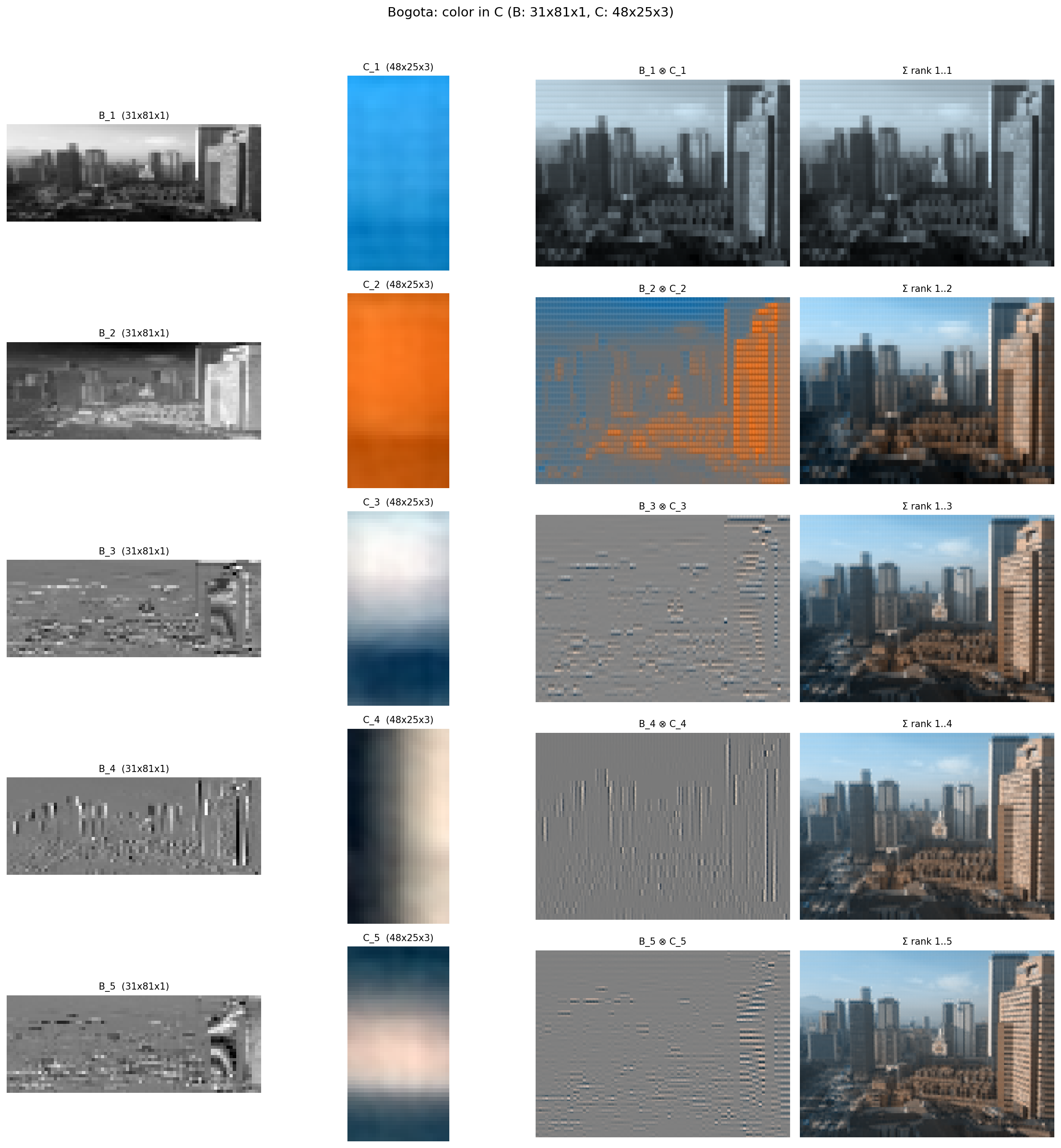
With color in \(C\), the picture changes. The first two modes are dedicated to capturing color: \(C_1\) is a solid blue (sky), \(C_2\) a solid orange (buildings and warm tones). Only from the third mode onward do we see the familiar progression of edges, lines, and texture. Color needs more rank budget when it lives in \(C\), because each term can only apply a single global tint:
Keep this intuition in mind: factor shapes control what gets captured at which scale, and rank determines how many dominant modes we retain. The same structure shows up when we compose convolutional layers.
From Convolution to Matrix Multiplication
A single convolutional layer takes an input \(X\) and slides a kernel \(W\) across it, computing a dot product at each position. For a single channel with stride equal to the kernel size (the simplest case), this is just:
\[y = vec(X)^T \cdot vec(W)\]Convolution is template matching: the output measures how well each input patch matches the kernel.
Composing Two Convolutions
Now stack two layers. The first with kernel \(W_1\) produces an intermediate activation; the second with kernel \(W_2\) operates on that. What single operation on the original input would produce the same result?
Under simplified assumptions (no activation function, single channel, stride equals kernel size), the composed operation is convolution with a single meta-kernel:
\[W_{meta} = W_2 \otimes W_1\]This is exact. The meta-kernel is the Kronecker product of the two individual kernels. If \(W_1\) is 3x3 and \(W_2\) is 3x3, the meta-kernel is 9x9. Each element of \(W_2\) scales a copy of \(W_1\), just like in image factorization:
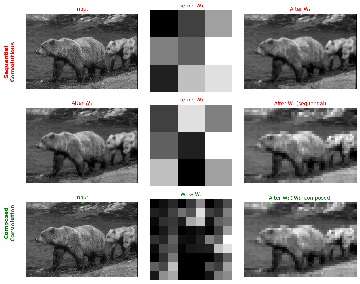
The top two rows show sequential convolution (input → \(W_1\) → intermediate → \(W_2\) → output). The bottom row shows a single convolution with \(W_2 \otimes W_1\) applied directly to the input. The outputs are identical.
The virtual matrix that maps input pixels to network output therefore has Kronecker structure by construction, which follows directly from composing convolutional layers rather than from any design choice.
What About ReLU?
Real networks have nonlinear activations between layers. For ReLU, the Kronecker structure still holds, with a twist.
ReLU passes positive activations unchanged and zeros out negative ones:
- Positive activations preserve the multiplicative relationship, so the Kronecker structure holds.
- Negative activations are equivalent to multiplying the weight by zero, masking out regions of the composed kernel.
The virtual matrix becomes data-dependent: different inputs produce different ReLU masks, which produce different composed kernels. Each input has its own virtual matrix, but each still has Kronecker structure underneath, modulated by the activation masks.
This gives us a useful way to think about ReLU: it selectively prunes the composed kernel, letting the network attend to different spatial patterns depending on the input. In deeper layers, a negative activation zeros out a region equivalent to the size of the composite kernel up to that point, so the pruning becomes increasingly coarse-grained.
Scaling to Multiple Channels
Real convolutions have multiple input and output channels. When composing two multi-channel layers, the meta-kernel becomes a sum of Kronecker products over the shared channels:
\[W_{meta} = \sum_{i=1}^{p} W_2^{(i)} \otimes W_1^{(i)}\]As a simpler example, composing two linear layers of shapes \(d_1 \times p\) and \(p \times d_2\) yields a matrix of rank at most \(p\), with the hidden dimension bounding the rank of the composition. The number of shared channels \(p\) plays the same rank-bounding role here.
This is the same form as the KFC and PHM layers from the previous post, but here it arises from composition, not from a design choice.
Relaxing the Stride Constraint
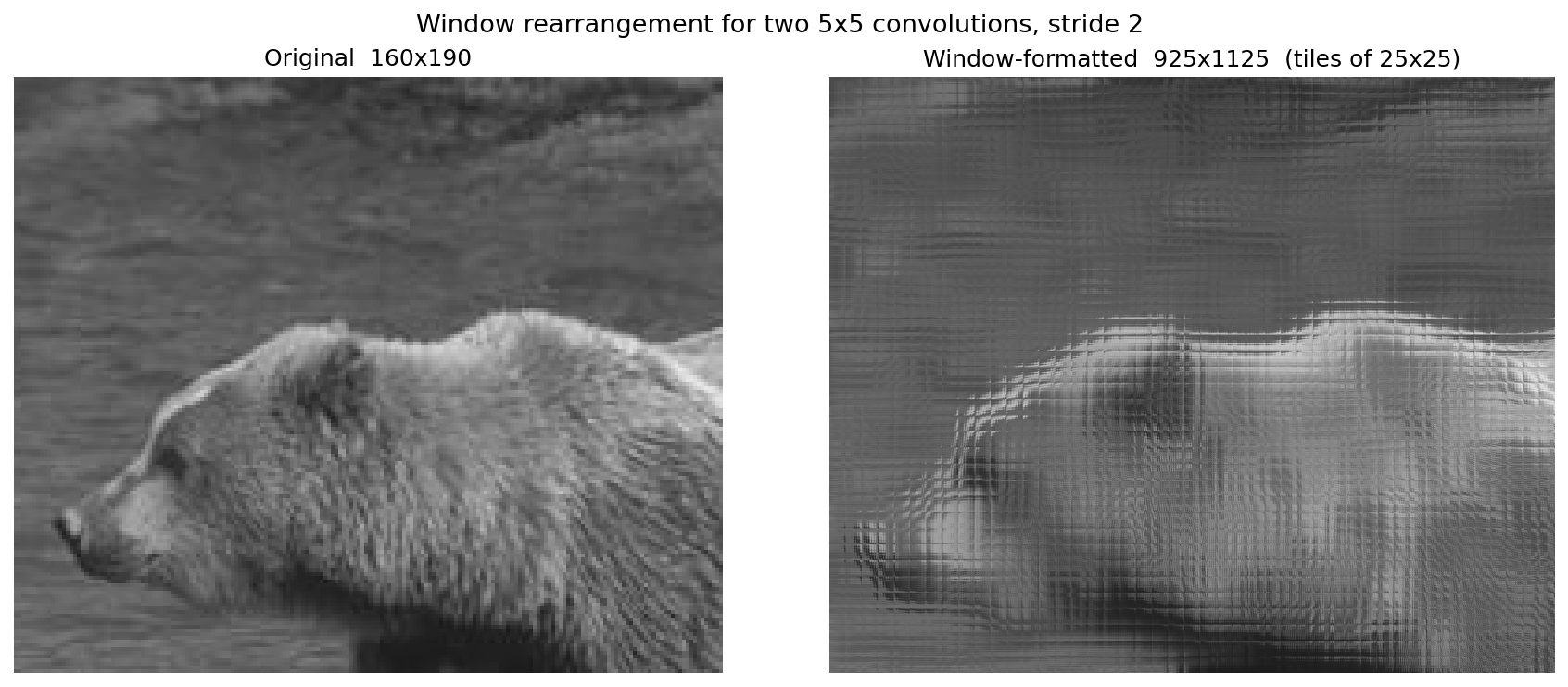
When the stride is smaller than the kernel size (the common case), input patches overlap. To handle this, the input must be rearranged into a window format where each element is a non-overlapping tile. The composed kernel still has Kronecker structure, but operates on the rearranged input.
The picture below shows this rearrangement for a crop around the bear’s face under two 5x5 convolutions with stride 2. Each sliding window is laid out as a non-overlapping \(25 \times 25\) tile (the outer product \(k_1 \cdot k_2\)), so the windowed representation is several times larger than the original. Because adjacent windows overlap by \(k - s = 3\) pixels, the same input pixels appear in many tiles, which shows up as a repeating texture in the rearranged image:
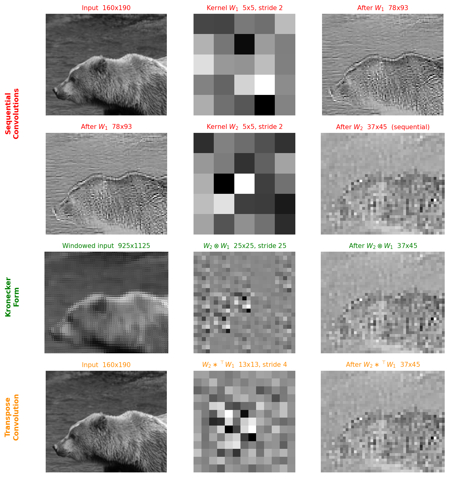
In practice, we never need to materialize the windowed input or the full Kronecker kernel explicitly. Given the adjoint relationship between convolution and transpose convolution, conv_transpose2d(W_2, W_1, stride=s_1) returns the composed kernel directly on the original image grid, applied at effective stride \(s_1 \cdot s_2\). The overlap bookkeeping implied by the window rearrangement is absorbed into the transpose-convolution operation itself.
The whole process can be observed in the figure below, which mirrors the earlier sequential-vs-composed picture, now for two 5x5 convolutions with stride 2. The top two rows run the layers sequentially. The third row applies the full Kronecker product \(W_2 \otimes W_1\) to the windowed input. The bottom row applies the transpose-convolution kernel \(W_2 \ast^\top W_1\) directly to the original input. All three paths produce the same output:
Kernel Size, Depth, and Rank
The connection between Kronecker products and SVD gives us a structural lens for understanding CNN architecture choices. Three relationships stand out:
Kernel size determines factor shapes
When two layers with kernel sizes \(k_1\) and \(k_2\) compose, the meta-kernel has size \(k_1 \cdot k_2\). The Kronecker product \(W_2 \otimes W_1\) has \(W_2\) as the “outer” factor (shape \(k_2 \times k_2\)) and \(W_1\) as the “inner” factor (shape \(k_1 \times k_1\)).
This parallels what we saw with image factorization: \(B\) controlled coarse shape and \(C\) controlled fine texture, with their dimensions determining the trade-off. In a CNN, the later layers’ kernels determine coarse spatial structure of the virtual matrix, while earlier layers’ kernels fill in fine-grained detail. The kernel size at each layer determines what spatial scales the network can represent.
Depth grows the kernel exponentially
Each additional layer multiplies the composed kernel size by its own kernel size. Three layers of 3x3 convolutions produce a 27x27 virtual kernel. Five layers produce 243x243. The composed kernel grows exponentially with depth.
Rather than compression, this shows how depth gives CNNs access to exponentially large receptive fields while only ever storing small kernels. A network with \(L\) layers of \(k \times k\) kernels has \(L \cdot k^2\) parameters but a virtual kernel of size \(k^L \times k^L\). The Kronecker structure is what makes this possible: it is an implicit factorization of an enormous matrix into a product of small ones.
Channels act as rank
The number of hidden channels \(p\) at each layer bounds the rank of the composed virtual matrix. Since the multi-channel composition is \(W_{meta} = \sum_{i=1}^{p} W_2^{(i)} \otimes W_1^{(i)}\), the rearranged matrix has rank at most \(p\).
This directly parallels SVD: a rank-\(p\) approximation captures \(p\) independent modes of variation. In the image decomposition, going from rank-1 to rank-10 dramatically improved reconstruction quality. In a CNN, more hidden channels means a higher-rank virtual matrix, which means more expressive class templates.
This gives a structural interpretation to the depth vs. width trade-off: depth controls the size of the virtual kernel (spatial extent), while width controls its rank (expressiveness). It also provides a bridge between nonlinear methods (neural networks with ReLU) and linear algebra (SVD): the virtual matrix of a CNN, despite being computed through nonlinear operations, has the same algebraic structure as a low-rank matrix factorization.
Visualizing the Virtual Matrix
The virtual matrix maps every input pixel to every output neuron. For classification, each output is a class, so each slice of the virtual matrix is a class-specific spatial template showing what pattern of input pixels that class responds to.
LeNet on MNIST
For a LeNet trained on MNIST (7 layers including pooling and FC), the data-independent composite kernels (ignoring activations) show clear digit-like templates:
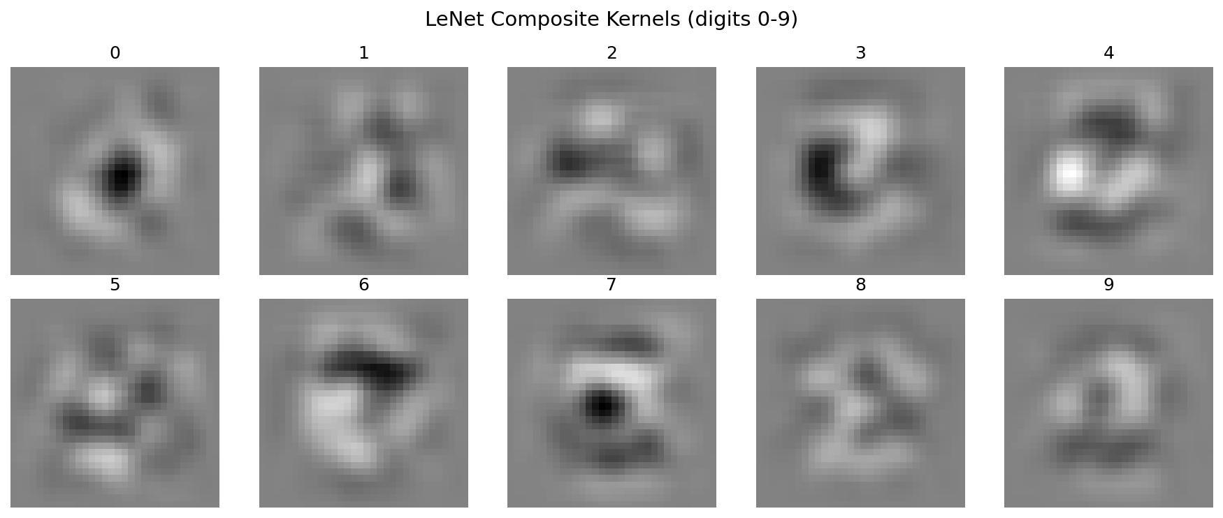
Each of the 10 templates visibly resembles the digit it classifies. Classification is template matching: the network computes a dot product between the input and each template, and the class with the highest response wins.
These templates emerge from composing many small kernels (5x5 convolutions, 2x2 pooling, fully connected layers). The network never explicitly learns a 32x32 template; the Kronecker structure of the composition produces one.
AlexNet on ImageNet
For a pretrained AlexNet (12 layers), the data-independent composite kernels (ignoring activations entirely) show dense, high-frequency grid patterns rather than recognizable objects:
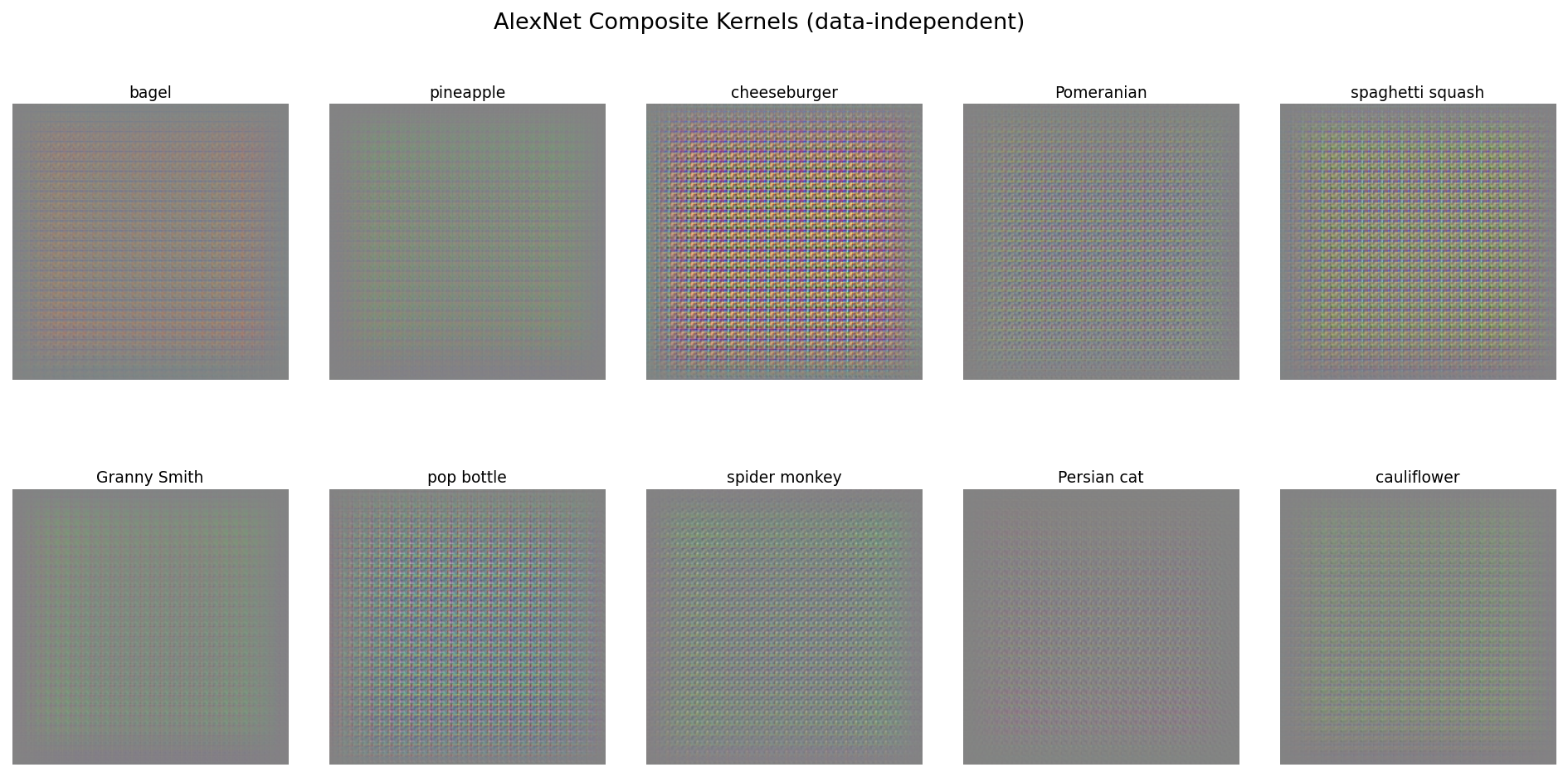
Without ReLU masking, the full Kronecker expansion of 12 layers produces a dense pattern dominated by the interaction of many small kernels.
The data-dependent version, using ReLU masks from an apple image, tells a different story. Class-specific patterns emerge, with object-like silhouettes shaped by which neurons fired for that particular input. This version is also numerically exact, in the sense that multiplying the input by this virtual matrix produces the same logits as running the input through the full network.
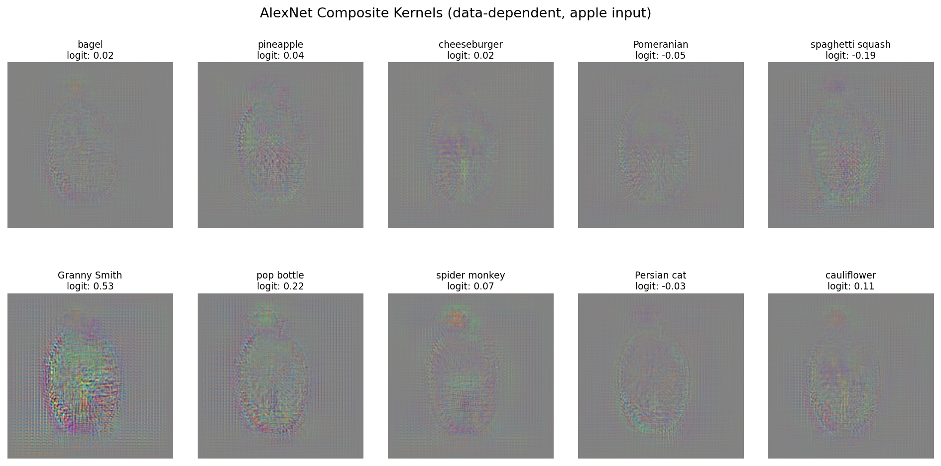
The contrast with LeNet is instructive. Depth matters, but so does data variance. MNIST digits are centered, roughly the same size, and have very low intra-class variance, so a single spatial template per class can go a long way. ImageNet classes, on the other hand, have enormous variation in pose, scale, lighting, and background. A “Granny Smith” can appear anywhere in the frame at any size. No single data-independent template could capture that variation, so the data-independent kernels end up as dense, uninterpretable patterns that need to encode all possible spatial configurations simultaneously. It is only when ReLU masks “carve” the template for a specific input that a coherent pattern emerges.
Activations and Effective Kernels by Layer
At each layer, the network has a set of channels, each detecting a specific spatial pattern. We can visualize two things side by side: the activation map (where and how strongly the pattern matched for a given input) and the effective kernel (the full-resolution pattern each channel has learned to detect, computed via Kronecker composition with ReLU masks).
The effective kernel at each layer accounts for all layers below it, composed via Kronecker expansion. At early layers (conv1), these are small 5x5 edge detectors embedded in the 32x32 input canvas. By the final layer (fc3), each of the 10 output channels has a full 32x32 template that, when dot-producted with the input, produces the class logit. ReLU masks make these templates input-specific: different digits activate different channels, producing different effective kernels. For convolutional layers where the effective kernel is smaller than the input (and varies by output position due to spatially varying ReLU masks), the visualization shows the kernel at the position of maximum activation for each channel.
Use the controls below to explore LeNet’s layers and digits:
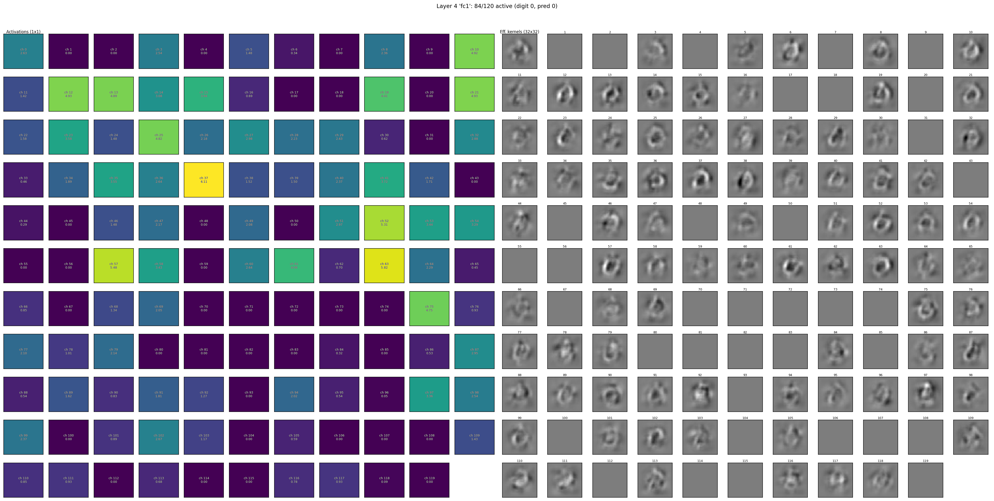
At conv1, each of the 6 channels is a small edge or gradient detector. By conv2, the 16 channels show larger oriented features (arcs, corners, crossings). At fc1, the 120 channels are full 32x32 patterns, many resembling partial digit strokes. At fc3, each of the 10 output channels is a class template whose dot product with the input gives the logit for that class.
The activation maps (left, viridis colormap) show where each pattern matched, while the effective kernels (right, grayscale) show what each channel detects. Comparing across digits reveals how ReLU selects different subsets of channels: the same kernel may be active for one digit and silent for another, changing the effective rank of the virtual matrix.
The same analysis applied to AlexNet on an apple image (showing up to 120 of each layer’s channels):
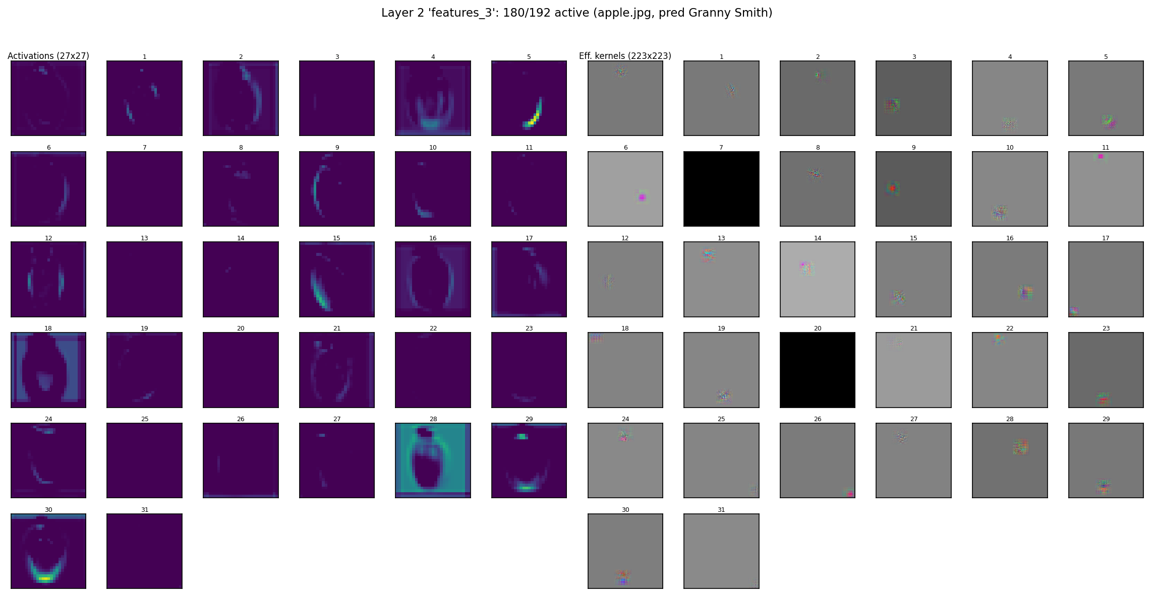
At conv1, the 64 channels show Gabor-like filters at various orientations and scales. By conv5 (L6), ReLU sparsity is dramatic: only 72 of 256 channels are active for this input, with most activations concentrated in a few channels. At the output layer (L10), each of the 1000 class channels has a scalar activation, with “Granny Smith” dominating.
Connection to Gradient Saliency
There is a precise mathematical equivalence between the Kronecker composition developed in this post and gradient-based saliency maps (Simonyan et al., 2013). Both compute the same object: the Jacobian of the network, \(\partial y / \partial X\).
The argument
For a ReLU network with a fixed input, every ReLU gate is either on (passing its input) or off (outputting zero). This makes the network a piecewise-linear function: within the activation region determined by the input, it is a single linear map from input pixels to output logits. The Jacobian \(J = \partial y / \partial X\) fully describes this linear map.
Saliency maps compute \(J\) via reverse-mode differentiation (backpropagation). The chain rule propagates gradients backward through each layer, multiplying by weight matrices and diagonal ReLU masks.
The Kronecker approach computes \(J\) via forward composition. At each layer, the effective kernel grows through Kronecker expansion (conv_transpose2d), and the ReLU mask zeros out channels whose activations were negative. The result is the same product of weight matrices and diagonal masks, just accumulated in the forward direction.
For two layers without ReLU, the Jacobian entry is:
\[J[o, c, r, s] = \sum_m \sum_{p,q} K_2[o,m,p,q] \cdot K_1[m,c, \; r - (i \cdot s_2 + p) \cdot s_1, \; s - (j \cdot s_2 + q) \cdot s_1]\]This is precisely the Kronecker expansion: conv_transpose2d places copies of \(K_1\) at stride-spaced positions, weighted by \(K_2\). With ReLU, each term is multiplied by the activation mask at the corresponding intermediate position:
The ReLU mask selects which Kronecker terms survive. The number of active channels at each cut point is the effective rank of the Jacobian at that point.
Numerical verification
To verify this equivalence, we compare three computations on a LeNet trained on MNIST:
- Kronecker composition: forward composition of conv kernels with ReLU masks folded in at each layer
- Gradient saliency:
torch.autogradcomputing \(\partial y[m, i, j] / \partial X\) - Forward pass: the actual network activation (ground truth)
All comparisons are at the center output position of each layer:
| Layer | Kronecker vs Saliency | Kronecker vs Forward | Saliency vs Forward |
|---|---|---|---|
| L0 conv1 | 0.00e+00 | 5.96e-08 | 5.96e-08 |
| L1 pool | 2.98e-08 | 1.79e-07 | 1.79e-07 |
| L2 conv2 | 8.94e-08 | 1.19e-06 | 1.19e-06 |
| L3 pool2 | 4.47e-08 | 3.58e-07 | 2.38e-07 |
| L4 fc1 | 8.20e-08 | 4.77e-07 | 4.77e-07 |
| L5 fc2 | 7.45e-08 | 9.54e-07 | 9.54e-07 |
| L6 fc3 | 1.19e-07 | 9.54e-07 | 1.91e-06 |
All differences are floating-point accumulation noise (\(\sim 10^{-6}\) to \(10^{-8}\)). The Kronecker composition and gradient saliency produce identical results at every layer.
What this means
Saliency maps have been used since 2013 as a visualization tool, but their internal structure has not been analyzed. The Kronecker perspective reveals that saliency maps inherit the same algebraic structure as composed convolutions: each is a sum of Kronecker products, one per active channel at any cut point, with ReLU determining how many terms survive.
This connects two lines of work that have developed independently:
- Kronecker factorization of composed convolutions, which reveals the rank and factor structure of the virtual matrix
- Gradient-based interpretability, which computes the input sensitivity of network outputs
They are computing the same object via different computational strategies: one goes forward composing weight matrices (Kronecker products), the other goes backward through the chain rule (backpropagation). The Kronecker view adds structural insight that backpropagation alone does not expose: the factorization into rank-1 Kronecker terms indexed by channels, the role of ReLU as rank selection, and the hierarchical multi-scale decomposition inherited from the layer-by-layer composition.
Looking Forward
The saliency equivalence is a satisfying place to arrive. What started as a purely algebraic observation about composed convolutions turns out to describe the same object that gradient-based interpretability has been computing since 2013. The Kronecker perspective gives saliency maps algebraic structure: a sum of Kronecker products whose rank and factors are determined by the network’s architecture and activation patterns.
This also resolves a practical limitation. The explicit Kronecker composition requires materializing per-position kernels, which grows prohibitively for large networks. But since the saliency map computes the same Jacobian via backpropagation, we can use autograd for efficiency while knowing that the result has Kronecker structure. The structure is there whether we construct it explicitly or not.
There are limitations. MaxPool is approximated as AvgPool, bias is ignored, and the analysis applies to piecewise-linear activations (ReLU, LeakyReLU) but not smooth nonlinearities (GELU, Swish) where the Jacobian is no longer a product of binary masks and weight matrices. Skip connections and normalization layers add terms that break the simple sum-of-Kronecker-products form, though extensions may be possible.
Open questions remain. What does the effective Kronecker rank (active channels after ReLU) tell us about a network’s utilization of its capacity? Can we prune channels that contribute little to the virtual matrix rank? How do the Kronecker factors differ for correctly vs. incorrectly classified inputs? And can this framework extend to attention mechanisms, where the “kernel” is itself data-dependent?
The code and experiments are available at github.com/santiag0m/kronecker.
References
- Van Loan, C. F., and N. Pitsianis. “Approximation with Kronecker Products.” Linear Algebra for Large Scale and Real-Time Applications. Springer, 1993.
- Zhou, S., Wu, J. N., Wu, Y., & Zhou, X. “Exploiting Local Structures with the Kronecker Layer in Convolutional Networks.” arXiv preprint arXiv:1512.09194 (2015).
- Zhang, A., et al. “Beyond Fully-Connected Layers with Quaternions: Parameterization of Hypercomplex Multiplications with \(1/n\) Parameters.” ICLR 2021.
- Zeiler, M. D., & Fergus, R. “Visualizing and Understanding Convolutional Networks.” European Conference on Computer Vision, 2014.
- Simonyan, K., Vedaldi, A., & Zisserman, A. “Deep Inside Convolutional Networks: Visualising Image Classification Models and Saliency Maps.” ICLR Workshop, 2014.
- Borji, A., & Lin, S. “White Noise Analysis of Neural Networks.” arXiv preprint arXiv:1912.12106 (2019).